Dynamic Programming vs Greedy

Dynamic programming is used to solve complex problems. Complex problems are broken into subproblems. Each stage of dynamic programming is a decision making process. At each stage a decision is taken that promotes optimization techniques for upcoming stages.

To carry-out Dynamic Programming following key functional working domain areas has to be considered:

Problem set
Methods used to define problem set
Recursion
Terminating condition
Overlapping Subproblems
Optimization technique

Problem Set should be concise. More concise the problem set is, more time and space efficiency is achieved. Problem set is generated using conditions, Conditions are used to filter problem set elements. Filter conditions are defined as per the requirement of the problem.

In Dynamic programming the solution formula is applied to the problem set which gives results. The solution formula is again applied to the result obtained and this process continues until the dynamic programming objective is obtained. Each time the solution formula is applied it must give the optimal value.

A problem can be treated as a dynamic programming problem if and only if the solution set itself represents the problem and contains conditions that lead to problem termination. It depends on the experience of the analyst that it identifies the problem as the dynamic programming problem and defines tight boundary conditions.

Dynamic programming is used in Mathematics, Computer programming, Bioinformatics etc.,

Following methods are often used to generate a problem set of dynamic programming:

Combinatorial Method
Generating functions
Transfer matrices
Recurrence relation
Graphical representation

Combinatorial method is based on binomial expression. Binomial expression is used to find possible filter conditions that may be used to form a problem set.

Generating functions from sequences. Sequences decide the condition and complexity of the problem. Using generating function recurrence of sequence is investigated based on which condition is decided to build the problem set.

Transfer matrices are used to develop relation matrices based on qualifying conditions. Conditions on which matrices are developed are pre-defined. If the problem is known at the very beginning then an optimal problem set can be obtained using simple matrix operations.

Recurrent relations define a sequence based on a predefined condition. In recurrence relation, next term is a function output of the previous terms. A problem may be defined using recurrence relation.

Graphical representation is used when the problem set consists of numerical values. A relation is developed among numerical values using graphs and this graph is used to form a problem set. Graphs depict relationships among two variables which themselves are constituent elements of the problem set. Relationships among variables are depicted using algebraic expressions.

Recursion in Dynamic Programming is used to define a problem set, a problem set is generated using conditions. Conditions to generate a problem set should be such that each element of the problem set is defined in terms of other elements of the problem set. When this is achieved it is termed as a recursive process. This recursive process is defined by recurrence relation. Using recurrence relation problem sets can be generated with minimum initial values and rules. In recursion logical operations should be performed in such a way that it does not lead to infinite execution of the function.

The most critical property of the problem set in dynamic programming is that it should be recursive. Each recursive set is a finite set and mathematical operations such as union and intersection on recursive sets are also recursive.

Terminating Conditions in recursive functions is important, if it is not executed it leads to infinite execution of recursive functions. Terminating conditions must be formulated to make minimum recursive calls. The minimum the recursive call the better is the time complexity of the dynamic programming.

Overlapping Subproblems in dynamic programming are recursive. Intersection of recursive sets is not null. To improve the efficiency of dynamic programming, execution of the intersection of problem subsets must be killed. This intersection of problem subsets is called Overlapping subproblems.

Overlapping of subproblems is a desirable characteristic of dynamic programming but repeated execution of overlapping subproblems is undesirable. To overcome this, storing results of subproblems is preferred in such a way that when the same subproblem is requested to execute again its saved results are used. This mechanism improves time complexity as well as space complexity.

Optimization Techniques in dynamic programming improves time and space complexity. Dynamic programming algorithms work for optimal solutions. Optimal solution is obtained using heuristics defined in the problem set, these heuristics depend on objectives to be achieved. In addition to this, optimization in terms of time and space complexity is achieved by using efficient data structures having well defined, efficient and effective operations.

Turing Machines

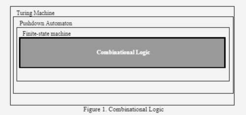
A Turing machine is an abstraction that operates on a set of rules. Turning machine examines input and its present state to make a decision to execute the next instruction or terminate. The Turing machine is the backbone of computer programming languages. Figure 1 gives insight into Dynamic Programming. In Figure 1 Combinational logic is the core Turing Machine and this combinational logic is used in dynamic programming to build recursive problem sets.

C Program to Implement Dynamic Programming (knapsack problem)

#include<stdio.h>
int m_ax(int a, int b) { return (a > b)? a : b; }
int knap_Sack(int W_k, int wt_k[], int val_k[], int n_k)
{
   int i, w_k;
   int K_p[n_k+1][W_k+1];
   for (i = 0; i <= n_k; i++)
   {
       for (w_k = 0; w_k <= W_k; w_k++)
       {
           if (i==0 || w_k==0)
               K_p[i][w_k] = 0;
           else if (wt_k[i-1] <= w_k)
                 K_p[i][w_k] = m_ax(val_k[i-1] + K_p[i-1][w_k-wt_k[i-1]],  K_p[i-1][w_k]);
           else
                 K_p[i][w_k] = K_p[i-1][w_k];
       }
   }
   return K_p[n_k][W_k];
}
int main()
{
    int i, n_k, val_k[20], wt_k[20], W_k;
    
    printf("Enter number of items:");
    scanf("%d", &n_k);
    
    printf("Enter value and weight of items:\n");
    for(i = 0;i < n_k; ++i){
     scanf("%d%d", &val_k[i], &wt_k[i]);
    }
 
    printf("Enter size of knapsack:");
    scanf("%d", &W_k);
    
    printf("%d", knap_Sack(W_k, wt_k, val_k, n_k));
    return 0;
}

Output:
Enter number of items:4

Enter value and weight of items:

120

23

135

45

235

56

678

56

Enter size of knapsack:100

798

Code Analysis

Number of input is taken from the user, It is the number of items that need to be put into the knapsack. Then user input weight and value for each item. Items are put into the knapsack in such a way that the total value is maximum and total weight is less than knapsack capacity.

In this program two user defined arrays are used - val[20] and wt[20].
Number of items to be put into the knapsack is taken from the user in integer variable n.

User defined function is used to put weights in a knapsack. Prototype of the function is:

                  int knap_Sack(int W_k, int wt_k[], int val_k[], int n_k)

In this function a two-dimensional integer type matrix is declared. Row of this matrix determines the number of items and the column determines the number of weights. This is dones as - int K_p[n_k+1][W_k+1];

weight and value array is passed to the knap_sack function. Two for loops are used in the knap_sack function and max function is used to find the maximum of value and weight. This is done by following programming instructions:

                                 for (i = 0; i <= n_k; i++)
                                {
                                      for (w_k = 0; w_k <= W_k; w_k++)
                                       {
                                             if (i==0 || w_k==0)
                                                   K_p[i][w_k] = 0;
                                              else if (wt_k[i-1] <= w_k)
                                                          K_p[i][w_k] = m_ax(val_k[i-1] + K_p[i-1][w_k-wt_k[i-1]], K_p[i-1][w_k]);
                                               else
                                                           K_p[i][w_k] = K_p[i-1][w_k];
                                        }
                                  }

User defined function m_ax uses a ternary operator to compare two values. This done by following instructions:

Greedy Algorithms

Greedy algorithm finds optimal solution. Greedy algorithm finds optimal choice at a particular instance of time without considering future outcomes of present decisions. Greedy algorithms find local optimum instead of global optimum.

Greedy algorithms execution is fast as compared to Divide & Conquer and Dynamic Programming. Some of the greedy algorithms includes:

Dijkstra’s Algorithm
Prim’s Algorithm
Huffman trees

Dijkstra’s algorithm is greedy. This algorithm finds the shortest path from a particular node to other nodes in the graph/network. The Dijkstra algorithm works on weighted directed graphs. In weighted directed graphs all the edges are assigned weight and direction.

Dijkstra algorithm is used in AI algorithms, Computer Networks and mobile Adhoc Networks.

Dijkstra algorithm works as follows:

Next node to be visited must have the shortest distance.
When a node is visited then its neighbouring nodes are recorded. From the neighbouring nodes find the distance to the root node. This is done by adding up the weights of the edges.

C Program to Implement Greedy Algorithm (Dijkstra Algorithm)

#include <limits.h>
#include <stdio.h>
#include <stdbool.h>


#define V_djk 9


int min_Distance(int d_ist_djk[], bool spt_Set[])
{

	int min_dijk = INT_MAX, min_index_djk;
	for (int v_djk = 0; v_djk < V_djk; v_djk++)
		if (spt_Set[v_djk] == false && d_ist_djk[v_djk] <= min_dijk)
			min_dijk = d_ist_djk[v_djk], min_index_djk = v_djk;

	return min_index_djk;
}


void printSolution(int d_ist_djk[ ])
{
	printf("Vertex \t\t Distance from Source\n");
	for (int i = 0; i < V_djk; i++)
		printf("%d \t\t %d\n", i, d_ist_djk[i]);
}


void dijkstra_djk(int graph[V_djk][V_djk], int src_djk)
{
	int d_ist_djk[V_djk]; 

	bool spt_Set[V_djk]; 

	
	for (int i = 0; i < V_djk; i++)
		d_ist_djk[i] = INT_MAX, spt_Set[i] = false;

	
	d_ist_djk[src_djk] = 0;

	
	for (int count_djk = 0; count_djk < V_djk - 1; count_djk++) {
		
		int u_djk = min_Distance(d_ist_djk, spt_Set);

		
		spt_Set[u_djk] = true;

		
		for (int v_djk = 0; v_djk < V_djk; v_djk++)

			
			if (!spt_Set[v_djk] && graph[u_djk][v_djk] && d_ist_djk[u_djk] != INT_MAX
				&& d_ist_djk[u_djk] + graph[u_djk][v_djk] < d_ist_djk[v_djk])
				d_ist_djk[v_djk] = d_ist_djk[u_djk] + graph[u_djk][v_djk];
	}

	
	printSolution(d_ist_djk);
}


int main()
{
	
	int graph_djk[V_djk][V_djk] = { { 0, 4, 0, 0, 0, 0, 0, 8, 0 },
						{ 14, 10, 18, 0, 0, 0, 0, 11, 0 },
						{ 10, 118, 0, 7, 0, 4, 0, 0, 2 },
						{ 20, 0, 7, 0, 9, 14, 0, 0, 0 },
						{ 30, 0, 0, 9, 0, 10, 50, 0, 0 },
						{ 0, 50, 4, 14, 10, 0, 2, 0, 0 },
						{ 0, 60, 0, 0, 50, 2, 0, 1, 6 },
						{ 8, 11, 0, 0,7, 0, 1, 0, 7 },
						{ 0, 0, 2, 0, 0, 0, 6, 7, 0 } };

	dijkstra_djk(graph_djk, 0);

	return 0;
}

Output:

Vertex 		 Distance from Source

0 		 0

1 		 4

2 		 15

3 		 22

4 		 15

5 		 11

6 		 9

7 		 8

8 		 15

The above code finds the shortest path using the Dijkstra algorithm which is greedy. Total of 9 vertices are taken. The program has four user defined functions -

 int min_Distance(int d_ist_djk[ ], bool spt_Set[ ] );
                 void printSolution(int d_ist_djk[ ])
                 void dijkstra_djk(int graph[V_djk][V_djk], int src_djk)

Function minDistance finds the vertex with minimum distance. This function has two parameters: first is integer type d_ist_djk[ ] array and second is bool variable array spt_Set[ ]. for loop is used to traverse all the vertices. Within the for loop if condition is used to check whether the vertex is traversed or not if it is not traversed and weight of the vertex is smaller than maximum integer value, then its weight is saved in the min variable. This program logic is implemented by following programming instructions:

 for (int v_djk = 0; v_djk < V_djk; v_djk++)
	if (spt_Set[v_djk] == false && d_ist_djk[v_djk] <= min_dijk)
	    min_dijk = d_ist_djk[v_djk], min_index_djk = v_djk;

Dijkstra algorithm is implemented in function :
                 void dijkstra_djk(int graph[V_djk][V_djk], int src_djk)

In this function for loop is used to find the shortest path for all vertices. Function minDistance is called from the for loop. The minDistance function returns the vertex with minimum weight from the available set of vertices. Programming instructions to implement this logic is:

 for (int count_djk = 0; count_djk < V_djk - 1; count_djk++) 
		int u_djk = min_Distance(d_ist_djk, spt_Set);

When the vertex is processed by the  boolean array spt_Set[u] it is set to true. This done by following programming instructions:


spt_Set[u_djk] = true;

d_ist_djk[ ] array is updated by for loop and if condition. Code  to implement this is:

for (int v_djk = 0; v_djk < V_djk; v_djk++)
    if (!spt_Set[v_djk] && graph[u_djk][v_djk] && d_ist_djk[u_djk] != INT_MAX
				&& d_ist_djk[u_djk] + graph[u_djk][v_djk] < d_ist_djk[v_djk])
				d_ist_djk[v_djk] = d_ist_djk[u_djk] + graph[u_djk][v_djk];

Conclusion

Following are the difference between Dynamic Programming and Greedy Algorithm:

Dynamic Programming	Greedy Algorithm
Dynamic programming ensures that it will produce optimal solutions.	Greedy Method does not ensure that it will produce an Optimal solution.
It requires more memory to perform its operations.	Memory requirement is less as compared to Dynamic Programming.
Time complexity is O(n2).	Time Complexity is O(n log n).